\(\newcommand{\newpara}{}
\newcommand{\nats}{\mathbb{N}}
\newcommand{\subcountawry}{\bf{When\ Counting\ Goes\ Awry}}
\newcommand{\seccountingstepscases}{\bf{Counting\ with\ Steps\ and\ Cases}}
\newcommand{\subalgfac}{\bf{Algebra:\ Factorials}}
\newcommand{\seccountingsubsets}{\bf{Counting\ Subsets}}
\newcommand{\secbitstrings}{\bf{Counting\ Bit\ Strings}}
\newcommand{\subhs}{Counting Handshakes}
\newcommand{\circled}[1]{\tikz[baseline=(char.base)]{\node[shape=circle,draw,inner sep=2pt] (char) {#1};}}
\newcommand{\xcircle}[1]{\circled{#1}}
\newcommand{\subdiscrete}{What is Discrete Mathematics?}
\newcommand{\sublearning}{Learning Discrete Mathematics}
\newcommand{\exerR}{Recap}
\newcommand{\subcountingawry}{When Counting Goes Awry}
\newcommand{\exerP}{Practice}
\newcommand{\subfactorials}{Algebra: Factorials}
\newcommand{\exerU}{Understand}
\newcommand{\subsubsetschoose}{Subsets and the Binomial Coefficients}
\newcommand{\exerE}{Explore}
\newcommand{\subcombinecount}{Combining Counting Techniques}
\newcommand{\subproofscountnosums}{Proof Format: Combinatorial Proof}
\newcommand{\subbitstrings}{Bit Strings}
\newcommand{\subcountbitstrings}{Number of Bit Strings}
\newcommand{\subrephrasingsubset}{Detour: Rephrasing the Question}
\newcommand{\subexplog}{Algebra: Exponential Notation and Logarithms}
\newcommand{\subbridges}{Crossing Bridges}
\newcommand{\subdefngraph}{The Definition of a Graph}
\newcommand{\subgraphcomp}{Graph Complements}
\newcommand{\subdegseq}{Degree Sequences}
\newcommand{\substdgraphs}{Standard Graphs}
\newcommand{\subadjmat}{The Adjacency Matrix of a Graph}
\newcommand{\subcolormaps}{Coloring Maps}
\newcommand{\subchromatic}{Coloring Graphs}
\newcommand{\subgraphconj}{Graph Conjectures}
\newcommand{\subplanarity}{Planarity}
\newcommand{\subisograph}{Isomorphic Graphs}
\newcommand{\subgraphtrees}{Subgraphs and Trees}
\newcommand{\subnonisograph}{Nonisomorphic Graphs}
\newcommand{\subgraphclassification}{Graph Classification}
\newcommand{\subrobots}{Detour: Robots}
\newcommand{\sublockers}{Opening and Closing Lockers}
\newcommand{\subevenodd}{Even and Odd Integers}
\newcommand{\subdivides}{Divisibility}
\newcommand{\subfractions}{Algebra: Equivalent Fractions}
\newcommand{\subdivalg}{The Division Algorithm, \fn{div}, and \fn{mod}}
\newcommand{\subpolys}{Algebra: Polynomials}
\newcommand{\subpffcases}{Proof Format: Proof by Cases}
\newcommand{\subnotlast}{Not Last Game}
\newcommand{\submod}{The Mod Clock}
\newcommand{\subzn}{The Integers mod $n$}
\newcommand{\subprimes}{Primes and Composites}
\newcommand{\subprimefact}{Prime Factorization}
\newcommand{\subcountdiv}{Detour: Listing and Counting Divisors}
\newcommand{\subgcd}{Greatest Common Divisor}
\newcommand{\subea}{The Euclidean Algorithm}
\newcommand{\subcoprime}{Coprime Integers}
\newcommand{\subandor}{And and Or}
\newcommand{\subpffandor}{Proof Formats: $\land$ and $\lor$ by Cases}
\newcommand{\subequivneg}{Logical Equivalence and Negations}
\newcommand{\subpffcontra}{Proof Format: Contradiction}
\newcommand{\subsetgame}{The Game SET}
\newcommand{\subquant}{Quantifiers}
\newcommand{\subpffquants}{Proof Formats: $\forall$ and $\exists$}
\newcommand{\subcex}{Negating Quantified Statements and Counterexamples}
\newcommand{\subifthen}{Promises: Conditional Statements}
\newcommand{\subpffifthen}{Proof Format: Direct Proof of $\to$}
\newcommand{\subnegcond}{Broken Promises: Negating Conditional Statements}
\newcommand{\subpfforimplication}{Proof Formats: Proof of $\lor$ Using Implication}
\newcommand{\subconv}{The Converse and Biconditional Statements}
\newcommand{\subpffiff}{Proof Format: $\leftrightarrow$}
\newcommand{\subcp}{The Contrapositive}
\newcommand{\subpffcp}{Proof Format: $\to$ Using the Contrapositive}
\newcommand{\subequiv}{Logical Equivalence}
\newcommand{\subneg}{Simplifying Negations}
\newcommand{\subinference}{Logical Inference}
\newcommand{\subinfsetsnumbers}{Infinite sets of numbers}
\newcommand{\subdefnfnnotation}{Function Notation and Vocabulary}
\newcommand{\subpiecewise}{Piecewise-defined Functions}
\newcommand{\subfndotgraphs}{Dot Diagrams and Graphs of Functions}
\newcommand{\subfloorceiling}{Floor and Ceiling}
\newcommand{\subnumberfn}{Number-theoretic Functions}
\newcommand{\subfngraphs}{Graph-theoretic Functions}
\newcommand{\subbitstringfunctions}{Functions Involving Bit Strings}
\newcommand{\suborderedpair}{Ordered Pairs and the Definition of Function}
\newcommand{\subpairing}{Pairings}
\newcommand{\subonetooneonto}{One-to-one and Onto}
\newcommand{\subperms}{Permutations}
\newcommand{\subinverses}{Inverse Functions}
\newcommand{\subpffunique}{Proof Format: Uniqueness}
\newcommand{\subdefnseq}{The Definition of Sequence}
\newcommand{\submodelseq}{Modeling with Explicitly-defined Sequences}
\newcommand{\subseqprimes}{Detour: Sequences Involving Primes}
\newcommand{\subelements}{Elements of a Set}
\newcommand{\subsetbuild}{Set-Builder Notation}
\newcommand{\subsetops}{Set Operations}
\newcommand{\subsubsets}{Subsets of a Set}
\newcommand{\subbsrepsubset}{Bit String Representation of Subsets}
\newcommand{\subsetsofsets}{Sets of Sets}
\newcommand{\subsetfn}{Detour: Set-theoretic Functions}
\newcommand{\subdefnpartition}{The Definition of Partition}
\newcommand{\subselfconj}{Conjugate Partitions}
\newcommand{\subbulgsol}{Collecting Coins}
\newcommand{\subcartprod}{The Cartesian Product of Sets}
\newcommand{\subfncartprod}{Functions Involving Cartesian Products}
\newcommand{\subdefnrelation}{Relations and Their Representations}
\newcommand{\subrelppty}{Properties of Relations}
\newcommand{\subequivclass}{Equivalence Relations and Equivalence Classes}
\newcommand{\subcongmod}{Congruence mod $n$}
\newcommand{\subhanoi}{The Towers of Hanoi}
\newcommand{\subrecdefseq}{Recursively-defined Sequences}
\newcommand{\subntr}{Modeling with Recursively-defined Sequences}
\newcommand{\subpffmathind}{Proof Format: Mathematical Induction}
\newcommand{\subalgind}{Algebra: Evaluating $f(n-1)$}
\newcommand{\subpffindseq}{Proof Format: Special Case of Mathematical Induction for Proving an Explicit Rule for a Recursively-defined Sequence}
\newcommand{\submatpowers}{Matrix Products and Powers}
\newcommand{\subpffindmatrix}{Proof Format: Special Case of Mathematical Induction for Proving an Explicit Formula for the Power of a Matrix}
\newcommand{\subgroups}{Finite Groups}
\newcommand{\subproperbs}{Proper Bit Strings}
\newcommand{\subrecsets}{Recursively-defined Sets}
\newcommand{\subrecgraphs}{Recursively-defined Graphs}
\newcommand{\subfib}{The Fibonacci Sequence and Higher Order Recursions}
\newcommand{\submodelhigher}{Modeling with Higher Order Recursions}
\newcommand{\subfibpatterns}{Detour: Fibonacci Patterns and Proof}
\newcommand{\subpffstrongind}{Proof Format: Strong Mathematical Induction}
\newcommand{\subhowmanysq}{Counting Squares}
\newcommand{\subfactrep}{Factorial Representations}
\newcommand{\subsigmapi}{Sum and Product Notation}
\newcommand{\subbaseb}{Base $b$ Representation}
\newcommand{\subbinary}{Binary Representation}
\newcommand{\subhex}{Hexadecimal Representation}
\newcommand{\subhexforbinary}{Hex as a Shorthand for Binary}
\newcommand{\subsumconj}{Sum Conjectures}
\newcommand{\subprodconj}{Product Conjectures}
\newcommand{\subsumfib}{Detour: Fibonacci Sums}
\newcommand{\subfactorpolys}{Algebra: Factoring Polynomials}
\newcommand{\subarithtri}{The Arithmetic Triangle}
\newcommand{\subpascalpatterns}{Patterns in the Arithmetic Triangle}
\newcommand{\subbinomthm}{The Binomial Theorem}
\newcommand{\subfactorialbinom}{Explicit Formula for Binomial Coefficients}
\newcommand{\subpffsumproofsind}{Proof Format: Special Case of Mathematical Induction for Proving Sum and Product Formulas}
\newcommand{\subpffcombsums}{Proof Format: Combinatorial Proof of Sums}
\newcommand{\subspecialsum}{Detour: Special Sums}
\newcommand{\subfracalg}{Algebra: Fraction Arithmetic}
\newcommand{\subhotelinf}{Hotel Infinity}
\newcommand{\subdefndiscrete}{The Definition of Discrete}
\newcommand{\seclisting}{Organized Listing}
\newcommand{\vocab}{\textbf}
\newcommand{\str}{\texttt}
\newcommand{\fn}{\texttt}
\newcommand{\bs}{\texttt}
\newcommand{\lt}{<}
\newcommand{\gt}{>}
\newcommand{\amp}{&}
\definecolor{fillinmathshade}{gray}{0.9}
\newcommand{\fillinmath}[1]{\mathchoice{\colorbox{fillinmathshade}{$\displaystyle \phantom{\,#1\,}$}}{\colorbox{fillinmathshade}{$\textstyle \phantom{\,#1\,}$}}{\colorbox{fillinmathshade}{$\scriptstyle \phantom{\,#1\,}$}}{\colorbox{fillinmathshade}{$\scriptscriptstyle\phantom{\,#1\,}$}}}
\)
Section3.2Standard Graphs and Representing Graphs
As we have seen, graphs can model many different situations. The drawing of a graph may lead to insights about the problem the graph is modeling. But the true power of graph models comes from a well-developed theory of graphs– facts that are true about all graphs, and the ability to implement algorithms on graphs using computer tools. We begin this section with some theory, the first theorem of graph theory. Next, graphs often have standard pieces, such as a row of connected vertices (a path), a circle of connected vertices (a cycle), or even a group of vertices that are all adjacent to each other (a complete graph). We introduce these and other standard graphs. To implement algorithms on a graph, we first need to enter the graph into a computer program. We introduce one such tool, the adjacency matrix of a graph.
One characteristic of a graph is the list of degrees of all the vertices. Some algorithms that run on graphs require a certain smallest or largest degree, or even that all the vertices have the same degrees. We define a few relevant terms.
Definition3.2.1Degree sequence and regular graphs.
The degree sequence of a graph is a list of the degrees of the vertices, including multiplicities. The degree sequence is usually written in nonincreasing order, which means largest to smallest. For example, the degree sequence of the classmates graph drawn in Figure 3.1.8 is
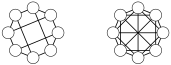
It is possible that all the vertices of a graph have the same degree. A graph is regular if all its vertices have the same degree. A regular graph is \(r\)-regular if every vertex has degree \(r\text{.}\) For example, the graph in Figure 3.2.2 is regular because every vertex has degree four.
In Activity 3.2.A(d), we observed a relationship between the degree sequence of \(S\) and the number of edges in \(S\text{:}\) if we add up the degrees of all the vertices in a graph, then we count each edge of the graph twice, because each endpoint of an edge counts that edge as part of their degree.
Perhaps this discussion reminds you of the Handshakes Puzzle Activity 1.1.A. If each person reports the number of handshakes they did and we calculate the sum, then we count each handshake twice. Therefore, that sum would be twice the number of handshakes.
The sum of the degrees of the vertices of a graph, counting multiplicities, is twice the number of edges. Equivalently, the number of edges of a graph is half of the sum of the degrees of the vertices.
In Activity 3.2.A(f), we considered whether there exists a 3-regular graph of order five. Use Theorem 3.2.5 to explain why there cannot exist such a graph.
Solution.
If there were such a graph, then the sum of the degrees would be
\begin{equation*}
3+3+3+3+3 = 15
\end{equation*}
which is an odd integer but, by Theorem 3.2.5, the sum of the degrees is twice the number of edges, which is an even integer. Since an integer cannot be even and odd (which we will formally prove in Theorem 4.2.2), such a graph is impossible.
Example3.2.7Is this list a degree sequence of a graph?
For each list of nonnegative integers, draw a graph with that degree sequence or explain why there cannot be a graph with that degree sequence.
\(5, 5, 3, 3, 3, 3\)Solution.
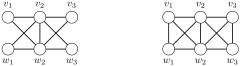
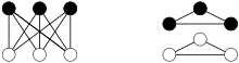
Let’s see what happens if we can draw a graph with this degree sequence. Note that there are six numbers listed, so our graph has six vertices. Therefore, each of the degree five vertices must be adjacent to all of the other five vertices. Therefore, our graph must start as shown on the left in Figure 3.2.8. The vertices \(v_2\) and \(w_2\) have degree five, but the other vertices only have degree two. We can increase their degree to three, as desired, by adding the edges \(\{v_1,w_1\}\) and \(\{v_3,w_3\}\text{,}\) for example, obtaining the graph drawn on the right in Figure 3.2.8. Thus, this list is the degree sequence of a graph.
Note that this graph is not the only graph with this degree sequence. We could have drawn edges between \(v_1\) and \(v_3\) and between \(w_1\) and \(w_3\text{,}\) for example.
Let’s see if we can draw a graph with this degree sequence. It would have six vertices. As before, the two vertices of degree five would each be adjacent to the other four vertices, as in the graph drawn on the left in Figure 3.2.8. But then all of the other vertices in our graph would already have degree at least two. That is a problem because our degree sequence lists a vertex of degree one. Thus, this list is not the degree sequence of any graph.
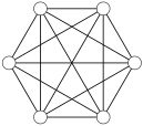
In Example 1.1.2 we drew a graph representing a group of six students shaking hands with each other, as drawn again in Figure 3.2.10. How many vertices does this graph have and what does that number mean in the story? How many edges does that graph have and what does that number mean in the story?
Solution.
The graph has six vertices that represent the six students. The graph has 15 edges that represent the 15 handshakes the group did.
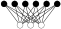
Six discrete mathematics students had just finished shaking hands and started studying when three first-year students wandered into the room. The discrete students thought it would be polite to greet each visitor by shaking hands. (Each discrete mathematics student shakes hands with each first-year student.) Draw a graph representing this new situation, only including the new handshakes.
Solution.
We draw the graph in Figure 3.2.11 and, as is common, we distinguish between the two types of students representing the discrete students with black vertices and the first-year students with white vertices. Which group is which color is not important and we do not have to color the vertices at all. Notice that there are \(6+3=9\) vertices representing the nine students and there are \(6\cdot3=18\) edges representing the 18 new handshakes.
Definition3.2.12Complete graphs and complete bipartite graphs.
A family of graphs is a set of graphs that share many properties. We might define a family in terms of a parameter such as \(s\text{.}\) In the name of the family, we often write that parameter as a subscript, a character written slightly smaller and lower. For example, the family of complete graphs \(K_s\) (pronounced “\(K\) sub \(s\)” ) for \(n\ge1\) are the graphs \(K_1\text{,}\)\(K_2\text{,}\)\(K_3\text{,}\) ….
For \(s \ge 1\) the complete graph (or handshake graph) with \(s\) vertices, denoted \(K_s\text{,}\) has an edge between every pair of vertices. The subscript \(s\) tells us the number of vertices. Note that “complete” starts with the sound of the letter “K”. For example, in Example 3.2.9(a), we drew the complete graph \(K_6\text{.}\)
For integers \(s,t \ge 1\text{,}\) the complete bipartite graph with \(s\) vertices of the first type (perhaps colored black in the drawing) and \(t\) vertices of the second type (perhaps colored white in the drawing), denoted \(K_{s,t}\) has an edge between each vertex of the first type and each vertex of the second type (and no other edges). For example, in Example 3.2.9(b), we drew the complete bipartite graph \(K_{6,3}\text{.}\)
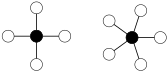
A special case of complete bipartite graphs is the star graphs \(K_{1,t}\) for \(t\ge1\text{.}\) For example, a star graph might model a corporate reporting structure such as a vice-president and their directors. Figure 3.2.13 shows drawings of \(K_{1,4}\) and \(K_{1,5}\) where we have drawn the white vertices in a circle around the central black hub vertex, as is customary.
Figure3.2.13.The stars \(K_{1,4}\) and \(K_{1,5}\text{.}\)
For each graph, count the number of vertices and edges and determine the degree sequence: the complete graph \(K_6\text{,}\) the complete bipartite graph \(K_{6,3}\text{,}\) and the star \(K_{1,5}\)Solution.
The complete graph \(K_6\) has six vertices and 15 edges. Every vertex has degree five, and so the degree sequence is \(5,5,5,5,5,5\text{.}\)
The complete bipartite graph \(K_{6,3}\) has nine vertices and 18 edges. The black vertices have degree three and the white vertices have degree six, so the degree sequence is \(6,6,6,3,3,3,3,3,3\text{.}\)
The star graph \(K_{1,5}\) has six vertices and five edges. Its hub vertex has degree five and the end vertices have degree one, so its degree sequence is \(5,1,1,1,1,1\text{.}\)
For \(s \ge 1\text{,}\) the path with \(s\) vertices, denoted \(P_s\text{,}\) has \(s\) vertices each adjacent to the next in a row. Officially, if the vertex set is \(\{v_1, v_2, \ldots,
v_s\}\text{,}\) then the edge set is
For \(s \ge 3\text{,}\) the cycle with \(s\) vertices, denoted \(C_s\text{,}\) has \(s\) vertices each adjacent to the next in a circle. Officially, if the vertex set is \(\{v_1, v_2, \ldots,
v_s\}\text{,}\) then the edge set is
For each graph, count the number of vertices and edges and write the degree sequence.
The paths \(P_4\) and \(P_5\text{.}\)Solution.
The path \(P_4\) has four vertices and three edges. The end vertices have degree one and the middle vertices have degree two. The degree sequence is \(2,2,1,1\text{.}\)
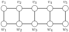
The ladder \(L_{2\times5}\) consists of two copies of the path \(P_5\) with \(5\) additional edges between each pair of corresponding vertices. Officially, if the vertex set is \(\{v_1,v_2,v_3,v_4,v_5,,w_1,w_2,w_3,w_4,w_5\}\text{,}\) then the edges are
For \(s \ge 3\text{,}\) the wheel, denoted \(W_s\text{,}\) consists of the cycle \(C_s\) with an additional hub vertex that is adjacent to each vertex in the cycle. For example, Figure 3.2.23 shows a drawing of \(W_3\text{.}\)
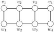
For \(t \ge 1\text{,}\) ladder, denoted \(L_{2\times t}\text{,}\) consists of two copies of the path \(P_t\) with \(t\) additional edges between each pair of corresponding vertices. Officially, if the vertex set is \(\{v_1,v_2,\ldots,v_t,w_1,w_2,\ldots,w_t\}\text{,}\) then the edges are
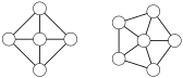
Draw the wheels \(W_4\) and \(W_5\text{.}\) For each graph count the number of vertices and edges, and list the degree sequence.
Solution.
Figure 3.2.26 shows a drawing of the graphs. The wheel \(W_4\) has five vertices and eight edges. The hub vertex has degree four and each of the outer vertices has degree three. Its degree sequence is \(4,3,3,3,3\text{.}\)
The wheel \(W_5\) has six vertices and ten edges. The hub vertex has degree five and each of the outer vertices has degree three. Its degree sequence is \(5,3,3,3,3,3\text{.}\)
Draw the ladder \(L_{2\times5}\text{,}\) count the number of vertices and edges, and list the degree sequence.
Solution.
Figure 3.2.27 shows a drawing of \(L_{2\times 5}\) which has ten vertices and thirteen edges. The four corner vertices have degree two and the rest of the vertices have degree three. Its degree sequence is \(3,3,3,3,3,3,2,2,2,2\text{.}\)
Graph models are especially useful because computers can work with graphs. 1
For example, \(\str{NetworkX}\) is a package of graph computation tools written in Python programming language.
One way for a computer to work with a graph is to list the vertices and edges. Another way is to list each vertex and its neighbors. An especially useful option represents a graph with a matrix (rectangular array) of \(\bs{0}\) s and \(\bs{1}\) s.
For any matrix \(A\text{,}\) the \(ij\)-entry of \(A\text{,}\) denoted \(A_{i,j}\text{,}\) is the entry in row \(i\) and column \(j\) of \(A\text{.}\) For example, if \(A= \left[ \begin{array}{cc} 1 \amp 2 \\ 3 \amp 4 \end{array} \right]\text{,}\) then \(A_{1,1}= 1\text{,}\)\(A_{1,2}= 2\text{,}\)\(A_{2,1}= 3\text{,}\) and \(A_{2,2}= 4\text{.}\)
To create an adjacency matrix\(A\) of a graph \(G\) with \(s\) vertices, we first list the vertices of \(G\) in order as \(v_1, v_2, \ldots, v_s\text{.}\) Then, the \(ij\)-entry of \(A\) equals \(\bs{1}\) if \(\{v_i,v_j\}\) is an edge and \(\bs{0}\) if \(\{v_i,v_j\}\) is not an edge. See Example 3.2.29 for an example.
Observe that \(A_{i,j}=A_{j,i}\text{,}\) so the adjacency matrix of a graph is symmetric. We can use this symmetry to build an adjacency matrix. For example, Example 3.2.29 once we knew that the first row of the adjacency matrix was \(\bs{010010}\text{,}\) it follows that the first column of the adjacency matrix was also \(\bs{010010}\text{.}\)
If the graph \(G\) has \(s\) vertices, then the adjacency matrix of \(G\) is an \(s \times s\) matrix, which means that it has \(s\) rows and \(s\) columns.
Notice that the matrix depends on the order of the vertices, here shown in alphabetical order. To obtain the first row of this matrix, we note that the vertex \(v_1\) is adjacent to the vertices \(v_2\) and \(v_4\text{.}\) Thus, \(A_{1,2}=\bs{1}\) and \(A_{1,4}=\bs{1}\) and the other entries in the first row are \(\bs{0}\text{.}\) Similarly, to get the second row, we note that \(v_2\) is adjacent to \(v_1\text{,}\)\(v_3\text{,}\)\(v_4\text{,}\) and \(v_5\text{.}\) Thus, \(A_{2,1}=\bs{1}\text{,}\)\(A_{2,3}=\bs{1}\text{,}\)\(A_{2,4}=\bs{1}\text{,}\) and \(A_{2,5}=\bs{1}\) and the other entries are \(\bs{0}\text{.}\) The other rows follow in a similar way.
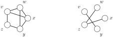
Determine the adjacency matrix for the graph \(G\) and its complement \(\overline{G}\) drawn in Figure 3.2.32 using the vertices in alphabetical order.
Figure3.2.32.The graph \(G\) and its complement \(\overline{G}\text{.}\)
Calculate the sum of the entries in each row of the adjacency matrix for \(G\) from (a). How are these sums related to the vertices of \(G\text{?}\) Explain.
Let \(G\) be a graph with adjacency matrix \(A\text{.}\)
Let \(v\) be a vertex in \(G\text{.}\) The degree of \(v\) is equal to the sum of the entries in the row (or column) of \(A\) corresponding to \(v\text{.}\)
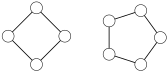
Hint: There are two possible graphs. One is six vertices in a circle. The other has two separate pieces. Check that each vertex of the graph you drew has degree two.
Hint: Your drawing should have three black vertices, four white vertices, and every possible black-white edge. The degree sequence is \(4,4,4,3,3,3,3\text{.}\)
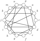
The Harary graphs \(H_{4,t}\) are a family of 4-regular graphs for \(t \ge 5\text{.}\) The graph \(H_{4,t}\) is constructed from the cycle \(C_t\) by adding an edge between each pair of vertices that are two edges apart in the cycle. For example, Figure 3.2.2 shows \(H_{4,6}\text{.}\)
In Section 3.1 Exercise 6, we defined a word graph whose vertices are the given words where two words are connected by an edge if one word can be changed to the other by making exactly one of the following changes.
For each graph listed, find a set of four words whose word graph is that graph. Be careful to check that if two vertices are not connected by an edge in the graph, then there is no way to change between those two words following the rules.
Hint: The adjacency matrix for \(C_5\) is the adjacency matrix for \(P_5\) with two more \(\bs{1}\) s. Say where those two additional \(\bs{1}\) s are.
Hint: The dividing lines create four blocks. Explain how each of the four blocks is constructed. For example, the upper left-hand block is a \(\bs{0}\text{.}\) The block to the right and block below it are each …. The lower right-hand block is …. Make sure to mention the adjacency matrix for \(C_5\text{.}\)
Describe how to construct the adjacency matrix for \(C_s\) using the adjacency matrix for \(P_s\text{.}\) Hint: look at your matrix from Exercise 1818.(a) and your answer to Exercise 1818.(c).