\(\newcommand{\newpara}{}
\newcommand{\nats}{\mathbb{N}}
\newcommand{\subcountawry}{\bf{When\ Counting\ Goes\ Awry}}
\newcommand{\seccountingstepscases}{\bf{Counting\ with\ Steps\ and\ Cases}}
\newcommand{\subalgfac}{\bf{Algebra:\ Factorials}}
\newcommand{\seccountingsubsets}{\bf{Counting\ Subsets}}
\newcommand{\secbitstrings}{\bf{Counting\ Bit\ Strings}}
\newcommand{\subhs}{Counting Handshakes}
\newcommand{\circled}[1]{\tikz[baseline=(char.base)]{\node[shape=circle,draw,inner sep=2pt] (char) {#1};}}
\newcommand{\xcircle}[1]{\circled{#1}}
\newcommand{\subdiscrete}{What is Discrete Mathematics?}
\newcommand{\sublearning}{Learning Discrete Mathematics}
\newcommand{\exerR}{Recap}
\newcommand{\subcountingawry}{When Counting Goes Awry}
\newcommand{\exerP}{Practice}
\newcommand{\subfactorials}{Algebra: Factorials}
\newcommand{\exerU}{Understand}
\newcommand{\subsubsetschoose}{Subsets and the Binomial Coefficients}
\newcommand{\exerE}{Explore}
\newcommand{\subcombinecount}{Combining Counting Techniques}
\newcommand{\subproofscountnosums}{Proof Format: Combinatorial Proof}
\newcommand{\subbitstrings}{Bit Strings}
\newcommand{\subcountbitstrings}{Number of Bit Strings}
\newcommand{\subrephrasingsubset}{Detour: Rephrasing the Question}
\newcommand{\subexplog}{Algebra: Exponential Notation and Logarithms}
\newcommand{\subbridges}{Crossing Bridges}
\newcommand{\subdefngraph}{The Definition of a Graph}
\newcommand{\subgraphcomp}{Graph Complements}
\newcommand{\subdegseq}{Degree Sequences}
\newcommand{\substdgraphs}{Standard Graphs}
\newcommand{\subadjmat}{The Adjacency Matrix of a Graph}
\newcommand{\subcolormaps}{Coloring Maps}
\newcommand{\subchromatic}{Coloring Graphs}
\newcommand{\subgraphconj}{Graph Conjectures}
\newcommand{\subplanarity}{Planarity}
\newcommand{\subisograph}{Isomorphic Graphs}
\newcommand{\subgraphtrees}{Subgraphs and Trees}
\newcommand{\subnonisograph}{Nonisomorphic Graphs}
\newcommand{\subgraphclassification}{Graph Classification}
\newcommand{\subrobots}{Detour: Robots}
\newcommand{\sublockers}{Opening and Closing Lockers}
\newcommand{\subevenodd}{Even and Odd Integers}
\newcommand{\subdivides}{Divisibility}
\newcommand{\subfractions}{Algebra: Equivalent Fractions}
\newcommand{\subdivalg}{The Division Algorithm, \fn{div}, and \fn{mod}}
\newcommand{\subpolys}{Algebra: Polynomials}
\newcommand{\subpffcases}{Proof Format: Proof by Cases}
\newcommand{\subnotlast}{Not Last Game}
\newcommand{\submod}{The Mod Clock}
\newcommand{\subzn}{The Integers mod $n$}
\newcommand{\subprimes}{Primes and Composites}
\newcommand{\subprimefact}{Prime Factorization}
\newcommand{\subcountdiv}{Detour: Listing and Counting Divisors}
\newcommand{\subgcd}{Greatest Common Divisor}
\newcommand{\subea}{The Euclidean Algorithm}
\newcommand{\subcoprime}{Coprime Integers}
\newcommand{\subandor}{And and Or}
\newcommand{\subpffandor}{Proof Formats: $\land$ and $\lor$ by Cases}
\newcommand{\subequivneg}{Logical Equivalence and Negations}
\newcommand{\subpffcontra}{Proof Format: Contradiction}
\newcommand{\subsetgame}{The Game SET}
\newcommand{\subquant}{Quantifiers}
\newcommand{\subpffquants}{Proof Formats: $\forall$ and $\exists$}
\newcommand{\subcex}{Negating Quantified Statements and Counterexamples}
\newcommand{\subifthen}{Promises: Conditional Statements}
\newcommand{\subpffifthen}{Proof Format: Direct Proof of $\to$}
\newcommand{\subnegcond}{Broken Promises: Negating Conditional Statements}
\newcommand{\subpfforimplication}{Proof Formats: Proof of $\lor$ Using Implication}
\newcommand{\subconv}{The Converse and Biconditional Statements}
\newcommand{\subpffiff}{Proof Format: $\leftrightarrow$}
\newcommand{\subcp}{The Contrapositive}
\newcommand{\subpffcp}{Proof Format: $\to$ Using the Contrapositive}
\newcommand{\subequiv}{Logical Equivalence}
\newcommand{\subneg}{Simplifying Negations}
\newcommand{\subinference}{Logical Inference}
\newcommand{\subinfsetsnumbers}{Infinite sets of numbers}
\newcommand{\subdefnfnnotation}{Function Notation and Vocabulary}
\newcommand{\subpiecewise}{Piecewise-defined Functions}
\newcommand{\subfndotgraphs}{Dot Diagrams and Graphs of Functions}
\newcommand{\subfloorceiling}{Floor and Ceiling}
\newcommand{\subnumberfn}{Number-theoretic Functions}
\newcommand{\subfngraphs}{Graph-theoretic Functions}
\newcommand{\subbitstringfunctions}{Functions Involving Bit Strings}
\newcommand{\suborderedpair}{Ordered Pairs and the Definition of Function}
\newcommand{\subpairing}{Pairings}
\newcommand{\subonetooneonto}{One-to-one and Onto}
\newcommand{\subperms}{Permutations}
\newcommand{\subinverses}{Inverse Functions}
\newcommand{\subpffunique}{Proof Format: Uniqueness}
\newcommand{\subdefnseq}{The Definition of Sequence}
\newcommand{\submodelseq}{Modeling with Explicitly-defined Sequences}
\newcommand{\subseqprimes}{Detour: Sequences Involving Primes}
\newcommand{\subelements}{Elements of a Set}
\newcommand{\subsetbuild}{Set-Builder Notation}
\newcommand{\subsetops}{Set Operations}
\newcommand{\subsubsets}{Subsets of a Set}
\newcommand{\subbsrepsubset}{Bit String Representation of Subsets}
\newcommand{\subsetsofsets}{Sets of Sets}
\newcommand{\subsetfn}{Detour: Set-theoretic Functions}
\newcommand{\subdefnpartition}{The Definition of Partition}
\newcommand{\subselfconj}{Conjugate Partitions}
\newcommand{\subbulgsol}{Collecting Coins}
\newcommand{\subcartprod}{The Cartesian Product of Sets}
\newcommand{\subfncartprod}{Functions Involving Cartesian Products}
\newcommand{\subdefnrelation}{Relations and Their Representations}
\newcommand{\subrelppty}{Properties of Relations}
\newcommand{\subequivclass}{Equivalence Relations and Equivalence Classes}
\newcommand{\subcongmod}{Congruence mod $n$}
\newcommand{\subhanoi}{The Towers of Hanoi}
\newcommand{\subrecdefseq}{Recursively-defined Sequences}
\newcommand{\subntr}{Modeling with Recursively-defined Sequences}
\newcommand{\subpffmathind}{Proof Format: Mathematical Induction}
\newcommand{\subalgind}{Algebra: Evaluating $f(n-1)$}
\newcommand{\subpffindseq}{Proof Format: Special Case of Mathematical Induction for Proving an Explicit Rule for a Recursively-defined Sequence}
\newcommand{\submatpowers}{Matrix Products and Powers}
\newcommand{\subpffindmatrix}{Proof Format: Special Case of Mathematical Induction for Proving an Explicit Formula for the Power of a Matrix}
\newcommand{\subgroups}{Finite Groups}
\newcommand{\subproperbs}{Proper Bit Strings}
\newcommand{\subrecsets}{Recursively-defined Sets}
\newcommand{\subrecgraphs}{Recursively-defined Graphs}
\newcommand{\subfib}{The Fibonacci Sequence and Higher Order Recursions}
\newcommand{\submodelhigher}{Modeling with Higher Order Recursions}
\newcommand{\subfibpatterns}{Detour: Fibonacci Patterns and Proof}
\newcommand{\subpffstrongind}{Proof Format: Strong Mathematical Induction}
\newcommand{\subhowmanysq}{Counting Squares}
\newcommand{\subfactrep}{Factorial Representations}
\newcommand{\subsigmapi}{Sum and Product Notation}
\newcommand{\subbaseb}{Base $b$ Representation}
\newcommand{\subbinary}{Binary Representation}
\newcommand{\subhex}{Hexadecimal Representation}
\newcommand{\subhexforbinary}{Hex as a Shorthand for Binary}
\newcommand{\subsumconj}{Sum Conjectures}
\newcommand{\subprodconj}{Product Conjectures}
\newcommand{\subsumfib}{Detour: Fibonacci Sums}
\newcommand{\subfactorpolys}{Algebra: Factoring Polynomials}
\newcommand{\subarithtri}{The Arithmetic Triangle}
\newcommand{\subpascalpatterns}{Patterns in the Arithmetic Triangle}
\newcommand{\subbinomthm}{The Binomial Theorem}
\newcommand{\subfactorialbinom}{Explicit Formula for Binomial Coefficients}
\newcommand{\subpffsumproofsind}{Proof Format: Special Case of Mathematical Induction for Proving Sum and Product Formulas}
\newcommand{\subpffcombsums}{Proof Format: Combinatorial Proof of Sums}
\newcommand{\subspecialsum}{Detour: Special Sums}
\newcommand{\subfracalg}{Algebra: Fraction Arithmetic}
\newcommand{\subhotelinf}{Hotel Infinity}
\newcommand{\subdefndiscrete}{The Definition of Discrete}
\newcommand{\seclisting}{Organized Listing}
\newcommand{\vocab}{\textbf}
\newcommand{\str}{\texttt}
\newcommand{\fn}{\texttt}
\newcommand{\bs}{\texttt}
\newcommand{\lt}{<}
\newcommand{\gt}{>}
\newcommand{\amp}{&}
\definecolor{fillinmathshade}{gray}{0.9}
\newcommand{\fillinmath}[1]{\mathchoice{\colorbox{fillinmathshade}{$\displaystyle \phantom{\,#1\,}$}}{\colorbox{fillinmathshade}{$\textstyle \phantom{\,#1\,}$}}{\colorbox{fillinmathshade}{$\scriptstyle \phantom{\,#1\,}$}}{\colorbox{fillinmathshade}{$\scriptscriptstyle\phantom{\,#1\,}$}}}
\)
Section3.5Classifying Graphs
A common theme across the sciences is to classify objects of a particular type. For example, how might we classify all trees with seven vertices? Since there are only finitely many, we can create a list of trees having seven vertices so that any tree with seven vertices is isomorphic to a tree on our list and no two trees on our list are isomorphic. We begin by discussing how to show that two graphs are not isomorphic.
Two graphs \(G\) and \(H\) are nonisomorphic, denoted \(G \ncong H\text{,}\) if they are not isomorphic. That is, if it is impossible to label the vertices of \(G\) and the vertices of \(H\) in such a way that \(G\) and \(H\) have the same vertices and the same edges.
This definition is not useful in writing proofs because it is subtle to prove that something is impossible. We might not find a way to label the vertices that shows that two graphs are isomorphic, but that does not prove that there is no labeling. We might not be able to visualize how one graph can be transformed into the other, but that does not mean that there is no way to do so. Let’s look at an example.
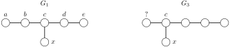
Let’s start with the labeling of \(G_1\) from Figure 3.4.9. The only degree 3 vertex in \(G_1\) is labeled \(c\text{.}\) That means \(c\) is the only vertex that appears in exactly three edges. The graph \(G_3\) has one degree 3 vertex, and if we want to produce the same edge list as \(G_1\text{,}\) that vertex needs to be labeled \(c\) to match, as shown in Figure 3.5.3.
Next, in \(G_1\text{,}\) the vertex \(c\) has exactly one neighbor with degree one, and it is labeled \(x\text{.}\) But in \(G_3\text{,}\) the vertex \(c\) has two neighbors with degree one. If we label one of those neighbors \(x\text{,}\) the other cannot be labeled (?). We are stuck. There is no common labeling. Therefore, \(G\) and \(K\) are not isomorphic.
Notice that we have identified a property that distinguishes \(G_1\) from \(G_3\text{,}\) namely \(G_1\) has exactly one vertex with degree three and that vertex has exactly one neighbor with degree one, but \(G_3\) does not have that property. This observation gives us a shorter proof that \(G_1\) and \(G_3\) are not isomorphic. After all, if they were the same graph, then they would have shared all graph-theoretic properties.
A graph invariant is a property \(\mathcal{P}\) that satisfies (\(\star\)) If a graph \(G\) has the property \(\mathcal{P}\) and \(G \cong H\text{,}\) then \(H\) also has the property \(\mathcal{P}\text{.}\) For example, “having exactly one degree three vertex” is a graph invariant.
Officially, we should prove that each of these properties is a graph invariant. Some properties that are not graph invariants are “is drawn as a 5-cycle plus edges” or “has adjacent vertices labeled \(a\) and \(b\)”. More generally, any property that refers to how a graph is drawn or labeled is not a graph invariant.
Remark3.5.6Using graph invariants to prove that two graphs are not isomorphic.
If two graphs are isomorphic, then they are the same graph, and therefore they must agree on all graph invariants. Equivalently 1
The statement \(\star\star\) is the contrapositive of \(\star\text{.}\) We will prove in Section 5.4 that a statement and its contrapositive are logically equivalent.
, for a graph invariant \(\mathcal{P}\text{,}\) (\(\star\star\)) If a graph \(G\) has the property \(\mathcal{P}\) but the graph \(H\) does not have the property \(\mathcal{P}\text{,}\) then \(G \ncong H\text{.}\) Therefore, to prove that graphs \(G\) and \(H\) are not isomorphic, we can find an invariant that \(G\) has but \(H\) does not or vice versa.
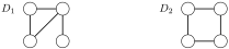
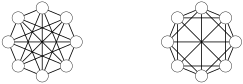
One reason \(D_1\) and \(D_2\) are nonisomorphic is that \(D_1\) has a vertex of degree one and \(D_2\) does not. Another reason is that they have different degree sequences: \(3,2,2,1\) for \(D_1\) versus \(2,2,2,2\) for \(D_2\text{.}\) Yet another reason is \(D_2\) contains a 4-cycle but \(D_1\) does not. And so on. Only one distinguishing graph invariant is needed. For any of these reasons, \(D_1 \ncong D_2\text{.}\)
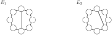
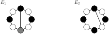
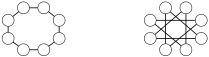
One reason \(E_1\) and \(E_2\) are nonisomorphic is that \(E_1\) contains two 5-cycles and \(E_2\) does not contain any 5-cycles. Another reason is that \(E_2\) can be 2-colored but \(E_1\) cannot, as shown in Figure 3.5.10.
Note that any 2-coloring of \(E_1\) would have to alternate around the 8-cycle but then the opposite end of the chord would have to be a third color. A different, quite complicated reason why \(E_1\) and \(E_2\) are nonisomorphic is that in \(E_2\) there is a pair of adjacent degree two vertices each of which has a degree three neighbor (the black vertex and white vertex to the right of the chord edge), but in \(E_1\) no pair of adjacent degree two both have degree three neighbors. For any of these reasons, \(E_1 \ncong E_2\text{.}\)
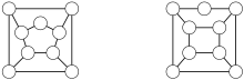
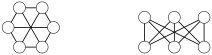
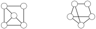
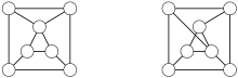
Check that the graphs drawn in Figure 3.5.12 have the same number of vertices, the same number of edges, and the same degree sequence and find a 4-cycle in each graph.
Classify all graphs with three vertices. That is, make a list of graphs having three vertices so that any graph with three vertices is isomorphic to a graph on our list and no two graphs on our list are isomorphic.
Solution.
There are four such graphs drawn in Figure 3.5.17. No two of these graphs are isomorphic because they have a different number of edges. You can (and should) convince yourself that there are no other options.
Classify all graphs with four vertices and three edges.
Solution.
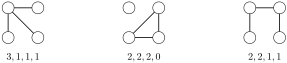
There are three such graphs drawn in Figure 3.5.18, labeled with their degree sequence. These graphs are not isomorphic because they have different degree sequences.
To check that this list is complete, suppose that we have a graph with four vertices and three edges. By Theorem 3.2.5, the sum of the degrees of the vertices is equal to twice the number of edges, which is \(2(3)=6\text{.}\) The degree sequence must be four nonnegative integers whose sum is equal to six. We consider the possibilities.
Case 1: The max degree is three. Notice that every other vertex is adjacent to the degree three vertex, and so the degree sequence is \(3,1,1,1\text{.}\) We get \(K_{1,3}\text{,}\) which is the graph on the left in Figure 3.5.18.
Case 2: The max degree must be two and there is an isolated vertex. The degree sequence would have to be \(2,2,2,0\text{.}\) Moreover, none of the three vertices having degree two can be adjacent to the isolated vertex, so the vertices having degree two must form a 3-cycle, and so we get the graph in the middle in Figure 3.5.18.
Case 3: The max degree is two and there is no isolated vertices. Then, the degree sequence is \(2, 2, 1, 1\text{.}\) The two degree two vertices must be adjacent to each other, and so we obtain a copy of \(P_4\text{,}\) which is the graph on the right in the graph in the middle of Figure 3.5.18.
Example3.5.19Using complements to classify graphs.
Classify all graphs with four vertices and two edges.
Solution.
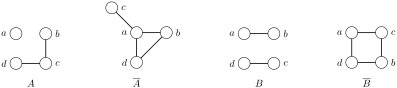
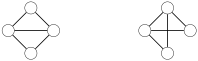
If the two edges share a common endpoint, then we get a graph \(A\) that has the path \(P_3\) and an isolated fourth vertex. Otherwise, we get a graph \(B\) that has two separate copies of \(P_2\text{.}\) Both are drawn in Figure 3.5.20.
Use the result of (a) to classify all graphs with four vertices and four edges.
Solution.
Since the complete graph \(K_4\) has six edges, the complement of any graph with four vertices and four edges must have four vertices and two edges. That is, the complement must be one of the two graphs we found in (a). The two graphs with four vertices and four edges are, therefore, \(\overline{A}\) and \(\overline{B}\) which are also drawn in Figure 3.5.20. We drew them without edge crossings just for fun, so look closely at the vertex labels.
Classify all trees with five vertices. That is, make a list of trees having five vertices so that any tree with five vertices is isomorphic to a tree on your list and no two trees on your list are isomorphic.
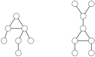
A connected graph is a robot if it contains one 3-cycle and no other cycles. For example, the graphs drawn in Figure 3.5.24 are robots. The left robot has seven vertices, and the right robot has eight.
How many different robots are there with six vertices. Hint: Organize your work based on how many vertices of the 3-cycle have edges beyond the 3-cycle — all three, two of them, or only one of them.
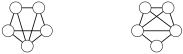
Hint: One answer is that the graph on the left has the degree sequence \(4,3,3,3,3\text{,}\) but the graph on the right has a different degree sequence. Can you find an easier answer?
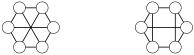
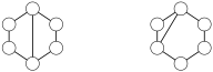
Use complements to show that the graphs drawn in Figure 3.5.28 are nonisomorphic by finding a graph invariant that distinguishes the complements of the two graphs.
The complement of the graph on the left is disconnected (it is two copies of \(C_3\)), but the graph on the right has a complement that is connected (it is isomorphic to \(C_6\)).
Hint: They are isomorphic. To prove that they are isomorphic, label the vertices so that they have the same vertices and the same edges. (It is not enough to show that they have many invariants in common.)
Hint: They are isomorphic. Label the vertices so that they have the same vertices and the same edges. Start with the degree two vertices, then their neighbors.
Hint: They are isomorphic. Their complements are a copy of \(P_2\) and two isolated vertices. Prove that the complements are isomorphic by labeling the vertices.
SubsubsectionExercises for 3.5.B Graph Classification
In these classification exercises, no justification is required, but make sure that your list is complete and that no two graphs on your list are isomorphic.
Hint: There are 11 total. One graph has no edges, and one graph has one edge. Example 3.5.19 lists all graphs with two edges and four edges. Example 3.5.16 lists the graphs with three edges. The graphs with five or six edges are the complements of graphs already on the list.
Hint: Small graphs are often given names that describe what they look like. Four of the answers are named the house, the kite, the dart, and the bowtie. (Please figure these out yourself, without peeking at resources!) There is one more possibility, but I do not know if it has a name.
Classify all trees with six vertices. Yes, this exercise repeats Activity 3.5.B(e). Hint: organize your work by drawing the longest possible path horizontally.
Classify all trees with seven vertices. Yes, this exercise repeats Activity 3.5.B(f). Hint: organize your work by drawing the longest possible path horizontally.
Classify all regular graphs with six vertices. Recall that in a regular graph, all vertices have the same degree \(r\text{.}\) Consider the cases \(r=0\text{,}\)\(r=1\text{,}\)\(r=2\text{,}\)\(r=3\text{,}\)\(r=4\text{,}\) and \(r=5\text{.}\)
Hint: There are one 0-regular, one 1-regular, and two 2-regular graphs. You can check if you have the correct number of 3-regular, 4-regular, and 5-regular by considering their complements.
Classify all trees with eight vertices. Hint: Organize your work by drawing the longest possible path horizontally. Another hint: there are 23 of them.
A connected graph is super-robot if it contains one 4-cycle and no other cycles. Draw a super-robot with six vertices, one with seven vertices, and one with eight vertices.
Classify all robots with seven vertices. No justification is required, but make sure that your list is complete and that no two robots on your list are isomorphic.
Super-robots were defined in Exercise 17. Draw all super-robots with eight vertices. No justification is required, but make sure that your list is complete and that no two super-robots on your list are isomorphic.