Section 6.4 Excursion: Permutations, Inverse Functions, and Uniqueness

We start this section by looking at permutations, which are bijections between a set and itself, and discuss the composition of permutations. Next, building on our examples with permutations, we define function composition and function inverses, in general. Lastly, we explore how to prove that a function is one-to-one and, more generally, a proof format for uniqueness proofs as well as existence and uniqueness proofs.

Subsection 6.4.A Permutations

Permutations are used in many applications. For example, they are used to describe the shuffling of a deck of cards, analyze sorting algorithms, and model gene sequencing. They are used in encryption and error-correction algorithms and for games such as anagrams, the sliding 15 puzzle, and Rubik’s Cubeβ„’. We start with the definition.

Definition 6.4.1 Permutation.

Β 
  1. A permutation is a function \(f:X \to X\) for some set \(X\) such that \(f\) is onto and one-to-one. In other words, a permutation is a bijection from a set to itself. Equivalently, a permutation is a function whose rule is a pairing of a set with itself. For example, the function \(h: \mathbb{R} \to \mathbb{R}\) defined by \(h(x) = 3x\) is a permutation, as we saw in ExampleΒ 6.3.34.
  2. We are often interested in a permutation of the set \(\{1,2,\ldots,n\}\) for some positive integer \(n\text{.}\) We can describe such permutations by listing the values, drawing the standard dot diagram, or using 2-line notation
    \begin{equation*} \alpha = \left(\begin{array}{ccc cc} 1 \amp 2 \amp 3 \amp \ldots \amp n \\ \alpha(1) \amp \alpha(2) \amp \alpha(3) \amp \ldots \amp \alpha(n) \end{array} \right) \end{equation*}
    For example, if \(\sigma: \{1,2,3,4\} \to \{1,2,3,4\}\) is the permutation defined by \(\sigma(1)=2\text{,}\) \(\sigma(2)=3\text{,}\) \(\sigma(3)=4\text{,}\) and \(\sigma(4)=1\text{,}\) then we write
    \begin{equation*} \sigma = \left(\begin{array}{ccc c} 1 \amp 2 \amp 3 \amp 4 \\ 2 \amp 3 \amp 4 \amp 1 \end{array} \right)\text{.} \end{equation*}
    In the 2-line notation, the first line is always \(1 2 3 \ldots n\) and the second line contains each of \(1, 2, 3, \ldots, n\) exactly once.
Permutations are often named with lowercase Greek letters.

Remark 6.4.2 Greek letters.

TableΒ 6.4.3 lists a few lowercase Greek letters commonly used for permutations.
Table 6.4.3. A few lowercase Greek letters commonly used for permutations
\(\alpha=\) alpha \(\beta=\) beta \(\gamma=\) gamma \(\delta=\) delta \(\epsilon=\) epsilon \(\mu=\) mu
\(\nu=\) nu \(\rho=\) rho \(\sigma=\) sigma \(\tau=\) tau \(\psi=\) psi \(\chi=\) chi
Let’s look more closely at permutations on \(\{1,2,3,4\}\text{.}\)

Example 6.4.4 Permutations on \(\{1,2,3,4\}\).

Β 
  1. Draw the dot diagram for the permutation \(\sigma = \left(\begin{array}{ccc c} 1 \amp 2 \amp 3 \amp 4 \\ 2 \amp 3 \amp 4 \amp 1 \end{array} \right)\text{.}\)
    Solution.
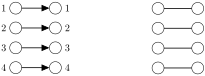
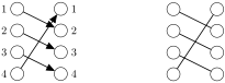
    FigureΒ 6.4.5 shows two versions of the dot diagram β€” the standard version on the left and an unlabeled version on the right.
    Figure 6.4.5. The dot diagram and unlabeled dot diagram for \(\sigma = \left( \begin{array}{ccc c} 1 \amp 2 \amp 3 \amp 4 \\ 2 \amp 3 \amp 4 \amp 1 \end{array} \right) \text{.}\)
  2. Is the identity function a permutation on \(\{1,2,3,4\}\text{?}\)
    Solution.
    The identity permutation \(i: \{1,2,3,4\} \to \{1,2,3,4\}\) is defined by \(i(n)=n\text{.}\) FigureΒ 6.4.6 shows the dot diagram of \(i\text{.}\) Since the function \(i\) is both onto and one-to-one with domain and codomain of \(\{1,2,3,4\}\text{,}\) the identity function \(i\) is a permutation. We can write
    \begin{equation*} i = \left(\begin{array}{ccc c} 1 \amp 2 \amp 3 \amp 4 \\ 1 \amp 2 \amp 3 \amp 4 \end{array} \right) \end{equation*}
    Figure 6.4.6. The dot diagram and unlabeled dot diagram for \(i = \left( \begin{array}{ccc c} 1 \amp 2 \amp 3 \amp 4 \\ 1 \amp 2 \amp 3 \amp 4 \end{array} \right) \text{.}\)
  3. How many permutations on \(\{1,2,3,4\}\) are there? Explain how you count.
    Solution.
    There are four choices for where the permutation maps one. Since permutations are one-to-one, there are three choices left for where the permutation maps two. Similarly, there are only two choices left for where the permutation maps three and then one choice for where the permutation maps four. Therefore there are \(4!\) permutations on the set \(\{1,2,3,4\}\text{.}\)
In ExampleΒ 6.4.4, we drew an unlabeled version of the dot diagrams where we omitted the vertex labels (always 1, 2, … \(n\) from top to bottom) and the arrows (always left-to-right). The unlabeled version can save writing and so we use it in our examples, but feel free to stick with the standard dot diagram if you prefer.
There is a natural way to combine permutations.

Definition 6.4.7 Permutation composition.

Β 
  1. For any permutations \(\alpha\) and \(\beta\) on \(\{1,2,3, \ldots,n\}\text{,}\) their composite \(\gamma\) is defined by \(\gamma(x) = \alpha(\beta(x))\text{.}\) We often write \(\alpha \circ \beta\) instead of \(\gamma\text{;}\) that is, \((\alpha \circ \beta)(x) = \alpha(\beta(x))\text{.}\) Notice in the composite \(\alpha \circ \beta\) that \(\beta\) is applied first and \(\alpha\) is applied second, which feels backward but is correct. For example, let
    \begin{equation*} \sigma = \left ( \begin{array}{cccc} 1 \amp 2 \amp 3 \amp 4 \\ 2 \amp 3 \amp 4 \amp 1 \end{array} \right ) \text{ and } \tau= \left ( \begin{array}{cccc} 1 \amp 2 \amp 3 \amp 4\\ 2 \amp 1 \amp 4 \amp 3 \end{array} \right )\text{.} \end{equation*}
    Then
    \begin{equation*} \sigma \circ \tau = \left ( \begin{array}{cccc} 1 \amp 2 \amp 3 \amp 4 \\ 3 \amp 2 \amp 1 \amp 4 \end{array} \right )\text{,} \end{equation*}
    as we see in ExampleΒ 6.4.8.
  2. For a permutation \(\alpha\text{,}\) the (\(n\)th) iterate of \(\alpha\) is the composite
    \begin{equation*} \alpha^n=\underbrace{\alpha \circ \alpha \circ \alpha \cdots \circ \alpha}_{n \text{ times } }\text{.} \end{equation*}
    For example, for that permutation \(\sigma\text{,}\) it turns out that
    \begin{equation*} \sigma^2=\sigma \circ \sigma = \left ( \begin{array}{cccc} 1 \amp 2 \amp 3 \amp 4 \\ 3 \amp 4 \amp 1 \amp 2 \end{array} \right )\text{,} \end{equation*}
    as we see in ExampleΒ 6.4.8.
Let’s check the examples from DefinitionΒ 6.4.7.

Example 6.4.8 Composing permutations.

Consider the permutations
\begin{equation*} \sigma = \left ( \begin{array}{cccc} 1 \amp 2 \amp 3 \amp 4 \\ 2 \amp 3 \amp 4 \amp 1 \end{array} \right ) \text{ and } \tau= \left ( \begin{array}{cccc} 1 \amp 2 \amp 3 \amp 4\\ 2 \amp 1 \amp 4 \amp 3 \end{array} \right ) \end{equation*}
  1. Calculate \(\sigma \circ \tau\text{.}\)
    Solution.
    We have
    \begin{align*} (\sigma \circ \tau)(1) \amp = \sigma(\tau(1))=\sigma(2)=3\\ (\sigma \circ \tau)(2) \amp = \sigma(\tau(2))=\sigma(1)=2\\ (\sigma \circ \tau)(3) \amp = \sigma(\tau(3))=\sigma(4)=1\\ (\sigma \circ \tau)(4) \amp = \sigma(\tau(4))=\sigma(3)=4 \end{align*}
    Thus
    \begin{equation*} \sigma \circ \tau = \left ( \begin{array}{cccc} 1 \amp 2 \amp 3 \amp 4 \\ 3 \amp 2 \amp 1 \amp 4 \end{array} \right )\text{.} \end{equation*}
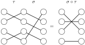
    There is a quicker way to compute this composite using the unlabeled dot diagrams shown in FigureΒ 6.4.9. To read this diagram, start with the uppermost dot on the left which represents 1. Moving right, follow the path to end on the third dot on the right which represents 3. Thus the composite maps 1 to 3. Repeat with each dot on the left following the path.
    Figure 6.4.9. The unlabeled dot diagram used to compute \(\sigma \circ \tau\) from ExampleΒ 6.4.8 (a).
  2. Calculate \(\tau \circ \sigma\text{.}\)
    Solution.
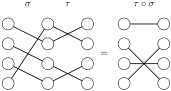
    Following the paths in FigureΒ 6.4.10 we get
    \begin{equation*} \tau \circ \sigma = \left ( \begin{array}{cccc} 1 \amp 2 \amp 3 \amp 4 \\ 1 \amp 4 \amp 3 \amp 2 \end{array} \right )\text{.} \end{equation*}
    Notice that the order mattered, in that \(\sigma \circ \tau \ne \tau \circ \sigma\text{.}\) That is, composition of permutations is not commutative.
    Figure 6.4.10. The unlabeled dot diagram used to compute \(\tau \circ \sigma\) from ExampleΒ 6.4.8 (b).
  3. Calculate \(\sigma^2=\sigma \circ \sigma\text{.}\)
    Solution.
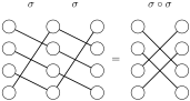
    Following the paths in FigureΒ 6.4.11 we get
    \begin{equation*} \sigma^2=\sigma \circ \sigma = \left ( \begin{array}{cccc} 1 \amp 2 \amp 3 \amp 4 \\ 3 \amp 4 \amp 1 \amp 2 \end{array} \right ) \end{equation*}
    Figure 6.4.11. The unlabeled dot diagram used to compute \(\sigma \circ \sigma\) from ExampleΒ 6.4.8 (c).
  4. Calculate \(\tau^2=\tau \circ \tau\text{.}\)
    Solution.
    Following the paths in FigureΒ 6.4.12 we get
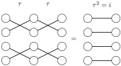
    \begin{equation*} \tau^2=\tau \circ \tau = \left ( \begin{array}{cccc} 1 \amp 2 \amp 3 \amp 4 \\ 1 \amp 2 \amp 3 \amp 4 \end{array} \right ) = i\text{,} \end{equation*}
    the identity permutation.
    Figure 6.4.12. The unlabeled dot diagram used to compute \(\tau \circ \tau\) from ExampleΒ 6.4.8 (d).
Notice that the composite of two permutations is another permutation. Now, it is your turn to work with permutations.

Activity 6.4.A Permutations.

Consider the permutations
\begin{equation*} \alpha = \left ( \begin{array}{ccc cc} 1 \amp 2 \amp 3 \amp 4 \amp 5 \\ 2 \amp 1 \amp 4 \amp 5 \amp 3 \end{array} \right )\text{ and } \mu= \left ( \begin{array}{ccc cc} 1 \amp 2 \amp 3 \amp 4 \amp 5 \\ 1 \amp 4 \amp 2 \amp 3 \amp 5 \end{array} \right ) \end{equation*}
  1. Evaluate \(\alpha(5)\text{,}\) \(\mu(3)\text{,}\) and \(\mu \circ \alpha(5)\text{.}\)
  2. Draw the dot diagram for \(\alpha\text{.}\)
  3. Add the dot diagram for \(\mu\) to your diagram, using the codomain of \(\alpha\) as the domain for \(\mu\text{.}\)
  4. Use your dot diagrams to calculate \(\mu \circ \alpha\text{.}\) Remember that \(\alpha\) goes first. Report your answer in 2-line notation.
  5. Check that your answers to (a) and (d) agree.
  6. Use dot diagrams to find a permutation \(\beta\) such that \(\beta \circ \alpha= i\text{,}\) the identity permutation. Remember that \(\alpha\) goes first.

Subsection 6.4.B Inverse Functions

How often have you done something on a computer, decided it was a mistake, and hit undo? As you may have learned (the hard way), some operations are invertible, meaning that they can be undone, and others are not. Let’s make this concept formal.

Definition 6.4.14 Inverse function.

Β 
  1. A function \(f: X \to Y\) is invertible if the equation \(f(x) = y\) has exactly one solution for each value of \(y\) in \(Y\text{.}\) For example, the function \(f: \mathbb{Z} \to \mathbb{Z}\) defined by \(f(n) = n+1\) is invertible because the equation \(f(n) = m\) is really \(n+1=m\) which has one solution, namely \(n=m-1\text{.}\) On the other hand, the function \(\fn{trim}: \mathbb{B}^* \to \mathbb{B}\) defined by \(\fn{trim}(b) =\) the bit string \(b\) without its last bit is not invertible because, for example, \(\fn{trim}(b) = \bs{101}\) has two solutions, namely \(b\)=\(\bs{1011}\) and \(b\)=\(\bs{1010}\text{.}\)
  2. For an invertible function \(f: X \to Y\text{,}\) the inverse function \(f^{-1}: Y \to X\) is defined by \(f^{-1}(y)\) is the unique solution of \(f(x)=y\text{.}\) That is, \(f^{-1}(y)=x\) exactly when \(f(x) = y\text{.}\) In this way, \(f^{-1}\) undoes \(f\text{.}\) Note that \(f^{-1}\) is pronounced as β€œ\(f\) inverse”. For example, if \(f: \mathbb{Z} \to \mathbb{Z}\) is defined by \(f(n) = n+1\text{,}\) then \(f^{-1}: \mathbb{Z} \to \mathbb{Z}\) is defined by \(f^{-1}(m) = m-1\text{.}\) We can think of the function \(f\) as adding one, and so its inverse \(f^{-1}\) undoes that operation by subtracting one.
A function \(f: X \to Y\) is invertible if the equation \(f(x) = y\) has exactly one solution for each value of \(y\) in \(Y\text{.}\) That is, if for each element \(y\) in \(Y\) there is exactly one element \(x\) in \(X\) such that \(f(x) = y\text{,}\) which means \(f\) is one-to-one and onto. Thus, \(f\) is invertible if (and only if) it is a bijection. We state this result as a theorem.
Since any permutation is a bijection, any permutation is invertible. Let’s find the inverse of a permutation.

Example 6.4.16 Inverse of a permutation.

Consider the permutation
\begin{equation*} \sigma = \left(\begin{array}{ccc c} 1 \amp 2 \amp 3 \amp 4 \\ 2 \amp 3 \amp 4 \amp 1 \end{array} \right)\text{.} \end{equation*}
Since \(\sigma\) is a permutation, it is one-to-one and onto. Thus, \(\sigma\) is invertible.
  1. Find the inverse \(\sigma^{-1}\text{.}\)
    Solution.
    We display our work in TableΒ 6.4.17.
    Table 6.4.17. Calculating the inverse of a permutation
    We know that We conclude that
    \(\sigma(1) = 2\) \(\sigma^{-1}(2)=1\)
    \(\sigma(2) = 3\) \(\sigma^{-1}(3)=2\)
    \(\sigma(3) = 4\) \(\sigma^{-1}(4)=3\)
    \(\sigma(4) = 1\) \(\sigma^{-1}(1)=4\)
    Thus
    \begin{equation*} \sigma^{-1} = \left(\begin{array}{ccc c} 1 \amp 2 \amp 3 \amp 4 \\ 4 \amp 1 \amp 2 \amp 3 \end{array} \right) \end{equation*}
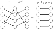
  2. Calculate \(\sigma^{-1} \circ \sigma\) using the dot diagrams.
    Solution.
    We show the dot diagrams in FigureΒ 6.4.18.
    Figure 6.4.18. Calculating \(\sigma^{-1} \circ \sigma\) using dot diagrams.
    Thus, \(\sigma^{-1} \circ \sigma = \left(\begin{array}{ccc c} 1 \amp 2 \amp 3 \amp 4 \\ 1 \amp 2 \amp 3 \amp 4 \end{array} \right) = i\text{.}\)
It is your turn to work with inverse functions.

Activity 6.4.B Invertible permutations.

Consider the permutations
\begin{equation*} \alpha = \left ( \begin{array}{ccc cc} 1 \amp 2 \amp 3 \amp 4 \amp 5 \\ 2 \amp 1 \amp 4 \amp 5 \amp 3 \end{array} \right ) \text{ and } \rho = \left ( \begin{array}{ccc cc} 1 \amp 2 \amp 3 \amp 4 \amp 5 \\ 2 \amp 3 \amp 4 \amp 5 \amp 1 \end{array} \right ) \end{equation*}
  1. Use that \(\alpha(4)=5\) to calculate \(\alpha^{-1}(5)\text{.}\)
  2. Write \(\alpha^{-1}\) in 2-line notation.
  3. Use dot diagrams to confirm that \(\alpha^{-1} \circ \alpha = i\text{.}\)
  4. Use dot diagrams to calculate \(\rho^2\text{,}\) \(\rho^3\text{,}\) \(\rho^4\text{,}\) and \(\rho^5\text{.}\) Report each answer in 2-line notation. (You can just keep adding to the same diagram.)
  5. Find \(\rho^{-1}\) and compare your answer to the powers of \(\rho\text{.}\) What do you notice?
  6. If \(\delta\) is a permutation and \(\delta^{10}=i\text{,}\) what can you say about \(\delta^{-1}\text{?}\)
It is not a coincidence that \(\sigma^{-1} \circ \sigma = i\text{,}\) the identity function. After all, the inverse function undoes the function. To state the general result, we first define the composition of the functions in general. (If you have seen calculus, the chain rule helped us take the derivative of the composite of functions.)

Definition 6.4.20 Function composition.

Β 
  1. Consider functions \(f: X \to Y\) and \(g: Y \to Z\text{.}\) Their composite function \(h: X \to Z\) is defined by \(h(x) = g(f(x))\text{.}\) We often write \(g \circ f\) instead of \(h\text{;}\) that is,
    \begin{equation*} (g \circ f)(x) = g(f(x))\text{.} \end{equation*}
    For example, if \(v: \mathbb{Z} \to \mathbb{Z}\) is defined by \(v(n) = n-1\) and \(w: \mathbb{Z} \to \mathbb{Z}\) is defined by \(w(n) = 2n\text{,}\) then
    \begin{equation*} (w \circ v)(n) = w(v(n)) = w(n-1) = 2(n-1) = 2n-2\text{.} \end{equation*}
    Note that
    \begin{equation*} (v \circ w)(n) = v(w(n)) = v(2n) = 2n-1\text{.} \end{equation*}
  2. If a function \(f:X \to X\) has the same set for its domain and codomain, then the (\(n\)th) iterate of \(f\) is the composite
    \begin{equation*} f^n=\underbrace{f \circ f \circ f \cdots \circ f}_{n \text{ times } }\text{.} \end{equation*}
    For example, if \(v: \mathbb{Z} \to \mathbb{Z}\) is defined by \(v(n) = n-1\text{,}\) then \(v^2: \mathbb{Z} \to \mathbb {Z}\) is defined by
    \begin{equation*} v^2(n) = v(v(n))=v(n-1) = (n-1)-1 = n-2 \end{equation*}
    and \(v^3: \mathbb{Z} \to \mathbb {Z}\) is defined by
    \begin{equation*} v^3(n) = v(v^2(n)) = v(n-2) = (n-2)-1 = n-3\text{.} \end{equation*}
    By the way, it is reasonable to conjecture that \(v^k: \mathbb{Z} \to \mathbb {Z}\) is defined by \(v^k(n) = n-k\) for any positive integer \(k\text{.}\)
For any invertible function \(f\text{,}\) \(f^{-1} \circ f=i_X\) where \(i_X\) is the identity function on the set \(X\) because
\begin{equation*} (f^{-1} \circ f)(x)=f^{-1}(f(x)) = f^{-1}(y) = x\text{.} \end{equation*}
Similarly, \(f \circ f^{-1}=i_Y\text{,}\) where \(i_Y\) is the identity function on the set \(Y\text{,}\) because
\begin{equation*} (f \circ f^{-1})(y) = f(f^{-1}(y)) = f(x) = y\text{.} \end{equation*}
We state this result.

Subsection 6.4.C Proof Format: Uniqueness

How do we prove that a function \(f: X \to Y\) is one-to-one or that a function is invertible? In this section, we look at how to prove uniqueness and also how to prove existence and uniqueness.
Ironically, there are two different proof formats for proving uniqueness. The first is direct.
There is an indirect method to prove uniqueness that does not require us to find \(k\text{.}\) How can we do that? An intuitive approach would be a proof by contradiction TheoremΒ 5.1.24. That is, we would suppose that \(P(n_1)\) and \(P(n_2)\) with \(n_1 \neq n_2\) and derive a contradiction. However, such proofs typically do not use the assumption that \(n_1 \neq n_2\text{,}\) and therefore can be rewritten without using contradiction. That is, we can prove if \(P(n_1)\) and \(P(n_2)\text{,}\) then \(n_1=n_2\text{.}\)
As usual, when we present new proof formats, we give you examples to copy and edit.

Activity 6.4.C Uniqueness proofs.

Β 
  1. Copy the following direct proof. For a fixed integer \(a\text{,}\) prove that the equation \(2x+1 = a\) has at most one integer solution.

    Proof.

    Assume
    \begin{equation*} 2x+1 = a\text{.} \end{equation*}
    Subtract one from each side of the equation to get
    \begin{equation*} 2x = a-1\text{.} \end{equation*}
    Divide each side of the equation by two to get
    \begin{equation*} x = \frac{a-1}{2}\text{.} \end{equation*}
    Thus, if \(x\) is a solution, then \(x = \frac{a-1}{2}\text{.}\) It follows that \(x = \frac{a-1}{2}\) is the only possible solution.
    Therefore, the equation \(2x+1=a\) has at most one integer solution, namely \(x = \frac{a-1}{2}\text{.}\)
    Note: There will be one solution if \(a\) is odd and \(\frac{a-1}{2}\) is an integer. There will be no solutions if \(a\) is even and \(\frac{a-1}{2}\) is not an integer.
  2. Edit the proof from (a) to prove that the equation \(3x-4=b\) has at most one integer solution.
  3. Copy the following indirect proof. For a fixed integer \(a\text{,}\) prove that the equation \(2x+1 = a\) has at most one integer solution.

    Proof.

    Assume that the integers \(n_1\) and \(n_2\) are each a solution of \(2x+1=a\text{.}\) Then
    \begin{equation*} 2n_1+1=a \text{ and } 2n_2+1=a. \end{equation*}
    Equating these expressions we get
    \begin{equation*} 2n_1+1 = 2n_2+1. \end{equation*}
    Subtract one from each side of the equation to get
    \begin{equation*} 2n_1 = 2n_2. \end{equation*}
    Divide each side of the equation by two to get \(n_1 = n_2\text{.}\) Therefore, the equation \(2x+1=a\) has at most one integer solution.
  4. Edit the proof from (c) to prove that the equation \(3x-4=b\) has at most one integer solution.
Recall that the one-to-one property was the uniqueness part of the definition of pairing DefinitionΒ 6.3.13. Thus, we can use TheoremΒ 6.4.23 to prove that a function is one-to-one. Recall from DefinitionΒ 6.3.28 that a function \(f: X \to Y\) is one-to-one if for each element \(y\) of \(Y\text{,}\) there is at most one element \(x \in X\) such that \(f(x) =y\text{.}\) Using the indirect approach from TheoremΒ 6.4.23, we can prove that a function is one-to-one by showing if \(f(x_1) = y\) and \(f(x_2)=y\text{,}\) then \(x_1=x_2\text{.}\) There is no reason to mention \(y\text{.}\) We can prove that a function is one-to-one by showing if \(f(x_1) = f(x_2)\text{,}\) then \(x_1=x_2\text{.}\) We can restate the definition of one-to-one using this observation.

Remark 6.4.25 Alternative definition of one-to-one.

Let \(f: X \to Y\) be a function. Then \(f\) is one-to-one exactly when it satisfies the following condition. For all elements \(x_1\) and \(x_2\) in \(X\text{,}\) if \(f(x_1) = f(x_2)\text{,}\) then \(x_1 = x_2\text{.}\)

Example 6.4.26 Prove function is one-to-one.

Prove that the function \(f: \mathbb{Z} \to \mathbb{Z}\) defined by \(f(n) = 2n+1\) is one-to-one, using RemarkΒ 6.4.25.
Solution.
Proof. Let \(n_1\) and \(n_2\) be integers. Assume \(f(n_1) = f(n_2)\text{.}\) By the definition of \(f\text{,}\) it follows that
\begin{equation*} 2n_1+1=2n_2+1. \end{equation*}
Subtract one from each side of the equation to get
\begin{equation*} 2n_1 = 2n_2\text{.} \end{equation*}
Divide each side of the equation by two to get
\begin{equation*} n_1 = n_2\text{.} \end{equation*}
Therefore, the function \(f: \mathbb{Z} \to \mathbb{Z}\) defined by \(f(n) = 2n+1\) is one-to-one.
We can combine proof formats for existence and uniqueness to prove that there exists a unique value of \(n\) such that \(P(n)\text{.}\) We begin with a quick notation.

Remark 6.4.27 Notation for uniqueness.

There exists a unique value of \(n\) such that \(P(n)\) is denoted \(\exists ! n ~ P(n)\text{.}\)
To prove that \(\exists ! n ~ P(n)\) we need to prove two things β€” first, that there is at least one \(n\) with \(P(n)\) and second, that there is at most one \(n\) with \(P(n)\text{.}\) The first proves existence, which we can do using TheoremΒ 5.2.14. The second proves uniqueness, which we can do directly using TheoremΒ 6.4.22.
Let’s look at an example.

Example 6.4.29 Proof that there exists a unique.

Prove that there exists a unique graph with three vertices and three edges.
Solution.
Proof. First, consider the cycle \(C_3\text{.}\) Note that \(C_3\) has three vertices and three edges.
Next, let \(G\) be a graph with three vertices and three edges. Say the vertices are \(u\text{,}\) \(v\text{,}\) and \(w\text{.}\) There are only three possible edges between these vertices: \(uv\text{,}\) \(uw\text{,}\) and \(vw\text{.}\) Since \(G\) has three edges, it must have exactly those edges. Thus \(G = C_3\text{.}\) Therefore, there is at most one graph with three vertices and three edges, namely \(C_3\text{.}\)

Subsection 6.4.D Exercises

Subsubsection Exercises for 6.4.A Permutations

1. Practice.

Consider the permutation with 2-line notation
\begin{equation*} \rho = \displaystyle \left ( \begin{array}{ccc ccc} 1 \amp 2 \amp 3 \amp 4 \amp 5 \amp 6 \\ 3 \amp 4 \amp 1 \amp 6 \amp 5 \amp 2 \end{array} \right ) \end{equation*}
  1. List \(\rho(1), \rho(2), \rho(3), \rho(4), \rho(5), \rho(6)\text{.}\)
  2. Draw the dot diagram for \(\rho\text{.}\)
Check.
  1. Hint: The list begins 3, 4, 1, ….
  2. Hint: The dot diagram should have an arrow from 1 to 3 and an arrow from 3 to 1. There is also an arrow straight across from 5 to 5.

2. Practice.

Calculate the composite \(\delta \circ \gamma\) where
\begin{equation*} \delta = \left ( \begin{array}{ccc} 1 \amp 2 \amp 3 \\ 1 \amp 3 \amp 2 \end{array} \right ) \text{ and } \gamma= \left ( \begin{array}{ccc} 1 \amp 2 \amp 3 \\ 3 \amp 1 \amp 2 \end{array} \right ) \end{equation*}
  1. First calculate the composite by evaluating \(\delta \circ \gamma(1)\text{,}\) \(\delta \circ \gamma(2)\text{,}\) and \(\delta \circ \gamma(3)\text{.}\) Write your answer in 2-line notation.
  2. Confirm your answer using the unlabeled dot diagrams.
Check.
Hint: Make sure to follow the instructions in each part.

3. Practice.

Use dot diagrams to compose the permutations written in 2-line notation. Report your answer in 2-line notation.
  1. \(\displaystyle \displaystyle \left ( \begin{array}{ccc c} 1 \amp 2 \amp 3 \amp 4 \\ 1 \amp 2 \amp 4 \amp 3 \end{array} \right ) \circ \displaystyle \left ( \begin{array}{ccc c} 1 \amp 2 \amp 3 \amp 4 \\ 1 \amp 3 \amp 2 \amp 4 \end{array} \right )\)
  2. \(\displaystyle \displaystyle \left ( \begin{array}{ccc c} 1 \amp 2 \amp 3 \amp 4 \\ 3 \amp 4 \amp 1 \amp 2 \end{array} \right ) \circ \displaystyle \left ( \begin{array}{ccc c} 1 \amp 2 \amp 3 \amp 4 \\ 2 \amp 3 \amp 4 \amp 1 \end{array} \right )\)
  3. \(\displaystyle \displaystyle \left ( \begin{array}{ccc c} 1 \amp 2 \amp 3 \amp 4 \\ 2 \amp 3 \amp 4 \amp 1 \end{array} \right ) \circ \displaystyle \left ( \begin{array}{ccc c} 1 \amp 2 \amp 3 \amp 4 \\ 4 \amp 1 \amp 2 \amp 3 \end{array} \right )\)
  4. \(\displaystyle \displaystyle \left ( \begin{array}{ccc c} 1 \amp 2 \amp 3 \amp 4 \\ 4 \amp 2 \amp 1 \amp 3 \end{array} \right ) \circ \displaystyle \left ( \begin{array}{ccc c} 1 \amp 2 \amp 3 \amp 4 \\1 \amp 2 \amp 3 \amp 4 \end{array} \right )\)
Check.
  1. \(\displaystyle \left ( \begin{array}{ccc c} 1 \amp 2 \amp 3 \amp 4 \\ 1 \amp 4 \amp 2 \amp 3 \end{array} \right )\) Hint: If you got \(\displaystyle \left ( \begin{array}{ccc c} 1 \amp 2 \amp 3 \amp 4 \\ 1 \amp 3 \amp 4 \amp 2 \end{array} \right )\) that is not correct. You composed the permutations in the opposite order. Remember, the one on the right goes first.
  2. Hint: The second line of the answer begins with 4.
  3. Hint: The answer is the identity permutation.
  4. Hint: The second line of the answer begins with 4.

4. Practice.

Use dot diagrams to calculate \(\rho^2\) and \(\rho^3\) when
\begin{equation*} \displaystyle \rho = \left ( \begin{array}{ccc ccc} 1 \amp 2 \amp 3 \amp 4 \amp 5 \amp 6 \\ 3 \amp 4 \amp 1 \amp 6 \amp 5 \amp 2 \end{array} \right )\text{.} \end{equation*}
Write the answers in 2-line notation.
Check.
Hint: \(\displaystyle \rho^2 = \left ( \begin{array}{ccc ccc} 1 \amp 2 \amp 3 \amp 4 \amp 5 \amp 6 \\ 1 \amp 6 \amp . \amp . \amp . \amp . \end{array} \right )\) and \(\displaystyle \rho^3 = \left ( \begin{array}{ccc ccc} 1 \amp 2 \amp 3 \amp 4 \amp 5 \amp 6 \\ 3 \amp 2 \amp . \amp . \amp . \amp . \end{array} \right )\text{.}\)

5. Understand.

Find an example of a nonidentity permutation on \(\{1,2,3,4,5\}\) that satisfies the stated condition, where \(i\) is the identity permutation on \(\{1,2,3,4,5\}\text{.}\) State your answer in 2-line notation.
  1. \(\displaystyle \alpha^2=i\)
  2. \(\displaystyle \beta^3 = i\)
  3. \(\gamma^4=i\) but \(\gamma^2 \neq i\)
  4. \(\displaystyle \delta^5 =i\)
Check.
  1. Hint: \(\alpha\) should swap two numbers, such as \(1 \to 2\) and \(2 \to 1\text{.}\) Send the other numbers to themselves.
  2. Hint: \(\beta\) should rotate three numbers cyclically, such as \(1 \to 2\text{,}\) \(2 \to 3\text{,}\) and \(3 \to 4\text{.}\)
  3. Hint: \(\gamma\) should rotate four numbers cyclically (and not just be swaps).
  4. Hint: \(\delta\) should rotate all five numbers cyclically.

7. Explore.

A transposition is a permutation that only switches two elements. For example \(\delta = \left ( \begin{array}{ccc} 1 \amp 2 \amp 3 \\ 1 \amp 3 \amp 2 \end{array} \right )\) is a transposition on \(\{1,2,3\}\text{.}\)
  1. Find the two other transpositions on \(\{1,2,3\}\text{.}\) Write your answers in 2-line notation and draw their dot diagrams.
  2. Draw the dot diagrams for each the transpositions on \(\{1,2,3,4\}\text{..}\)
  3. How can you tell from the dot diagram if a permutation is a transposition?
  4. How many transpositions on \(\{1,2,3, \ldots, n\}\) are there? Explain briefly.
Check.
  1. Hint: Another is \(\left ( \begin{array}{ccc} 1 \amp 2 \amp 3 \\ 2 \amp 1 \amp 3 \end{array} \right )\)
  2. Hint: There are six of them. Think about which pair of numbers is switched.
  3. Hint: Most of the lines are horizontal. What else do you see in the dot diagram?
  4. Hint: How many ways are there to choose the two numbers out of \(n\) to swap?

Subsubsection Exercises for 6.4.B Inverse Functions

8. Practice.

Use dot diagrams to calculate the inverse of each permutation. Write the answer in 2-line notation.
  1. \(\displaystyle \displaystyle \delta = \left ( \begin{array}{ccc} 1 \amp 2 \amp 3 \\ 1 \amp 3 \amp 2 \end{array} \right )\)
  2. \(\displaystyle \gamma= \left ( \begin{array}{ccc} 1 \amp 2 \amp 3 \\ 3 \amp 1 \amp 2 \end{array} \right )\)
  3. \(\mu= \displaystyle \left ( \begin{array}{ccc cc} 1 \amp 2 \amp 3 \amp 4 \amp 5 \\ 1 \amp 4 \amp 2 \amp 3 \amp 5 \end{array} \right )\text{.}\)
  4. \(\displaystyle \displaystyle \rho = \left ( \begin{array}{ccc ccc} 1 \amp 2 \amp 3 \amp 4 \amp 5 \amp 6 \\ 3 \amp 4 \amp 1 \amp 6 \amp 5 \amp 2 \end{array} \right )\)
Check.
  1. Hint: \(\delta\) is its own inverse.
  2. \(\displaystyle \displaystyle \gamma^{-1} = \left ( \begin{array}{ccc} 1 \amp 2 \amp 3 \\ 2 \amp 3 \amp 1 \end{array} \right )\)
  3. Hint: Check your answer by composing \(\mu^{-1} \circ \mu\text{.}\) You should get the identity.
  4. Hint: Check your answer by composing \(\rho^{-1} \circ \rho\text{.}\)

10. Understand.

Β 
  1. Draw dot diagrams for each of the six permutations on \(\{1,2,3\}\text{.}\) You do not need to label your dot diagrams.
  2. For each of those six permutations, state what its inverse permutation is. Hint: A permutation can be its own inverse.
Check.
  1. Hint: There are two that send \(1 \to 1\text{,}\) two that send \(1 \to 2\text{,}\) and two that send \(1 \to 3\text{.}\)
  2. Hint: Four of them are their own inverses. The remaining two are inverses of each other.

11. Understand.

Consider the functions \(\fn{trim}: \mathbb{B}^* \to \mathbb{B}\) defined by \(\fn{trim}(b) =\) the bit sting \(b\) without its last bit and \(\fn{append}:\mathbb{B} \to \mathbb{B}^*\) defined by \(\fn{append}(b)=b\bs{1}\text{,}\) literally the bit string \(b\) with a \(\bs{1}\) added to the right.
  1. Calculate \((\fn{append} \circ \fn{trim})(\bs{1010})\text{.}\)
  2. When is \((\fn{append} \circ \fn{trim})(b)=b\text{?}\)
  3. Calculate \((\fn{trim} \circ \fn{append})(\bs{1010})\text{.}\)
  4. When is \((\fn{trim} \circ \fn{append})(b)=b\text{?}\)
Check.
  1. Hint: You should not get \(\bs{1010}\text{.}\)
  2. Hint: It depends on the last bit of \(b\text{.}\)
  3. Hint: You should get \(\bs{1010}\text{.}\) Make sure you show work.
  4. Hint: Figure out what \(\fn{append}(b)\) is first.

12. Understand inverse of piecewise function.

Consider the function \(f: \mathbb{N} \to \mathbb{N}\) defined by
\begin{equation*} f(n) =\left\{ \begin{array}{cl} n+1 \amp \text{ if } n \text{ is even } \\ n-1 \amp \text{ if } n \text{ is odd } \end{array} \right.\text{.} \end{equation*}
The dot diagram for \(f\) is shown in FigureΒ 6.3.20.
  1. Calculate \(f^2(3)\) and \(f^2(6)\text{.}\)
  2. It turns out that \(f\) is a bijection. What is its inverse function?
Check.
  1. Hint: \(f^2(3) = f(f(3))=f(2)=\text{?}\)
  2. Hint: What is \(f^2\text{?}\) That tells you what \(f \circ f\) equals.

13. Understand.

Β 
  1. The function \(g: \mathbb{R} \to \mathbb{R}\) is defined by \(g(x) = ax\text{,}\) where \(a\) is a nonzero constant. Calculate \(g^2(x)\text{,}\) \(g^3(x)\text{,}\) and \(g^4(x)\) and make a conjecture about \(g^k(x)\) in general.
  2. The function \(f: \mathbb{Z} \to \mathbb{Z}\) is defined by \(f(n) = n + c\) where \(c\) is constant. Calculate and simplify \(f^2(n)\text{,}\) \(f^3(n)\text{,}\) and \(f^4(n)\text{.}\) Make a conjecture about \(f^k(n)\) in general.
Check.
  1. Hint: \(g^2(x) =g(g(x))=g(ax)=a(ax) =\text{?}\)
  2. Hint: \(f^2(n)=f(f(n))=f(n+c)=(n+c)+c=\text{?}\)

15. Explore.

Suppose \(f:X \to X\) is a bijection and, as usual, write \(i:X \to X\) for the identity function on \(X\text{.}\)
  1. If \(f^2=i\text{,}\) what does that tell you about \(f^{-1}\text{?}\)
  2. If \(f^3=i\text{,}\) what does that tell you about \(f^{-1}\text{?}\)

Subsubsection Exercises for 6.4.C Proof Format: Uniqueness

18.

{Understand} Prove there exists a unique rational solution to the equation \(2x + a = 2b\) for any integers \(a\) and \(b\text{.}\) Hint: Use TheoremΒ 6.4.28.
Check.
Hint: Before writing the proof, solve for \(x\) in terms of \(a\) and \(b\text{.}\) The proof has two parts. In the first part, consider \(x =\) (the answer you found). Evaluate \(2x + a\) when \(x=\) your answer and simplify to get \(2b\text{.}\) In the second part, show how you solved the equation.

20. Explore.

In this exercise, we prove the uniqueness of the remainder in the Division Algorithm TheoremΒ 4.2.2. To start the proof, we assume that \(a = nq_1+r_1\) and \(a = nq_2 + r_2\) for some integers \(a,n,q_1,r_1,q_2,r_2\) with \(n \ne4q 0\text{,}\) \(0 \le r_1 \lt n\text{,}\) and \(0 \le r_2\lt n\text{.}\) It is not a loss of generality to assume \(r_1 \ge r_2\text{.}\)
  1. Set the two expressions for \(a\) equal to each other and solve to prove that \(n \div (r_1-r_2)\text{.}\)
  2. Explain why \(0 \le r_1-r_2 \lt n\text{.}\)
  3. How can parts 20.(a) and 20.(b) both be true? What does your conclusion tell you about \(r_1\) and \(r_2\text{?}\)